Introduction to CFD - compressible gas dynamics

This blog serves as a friendly yet practical guide to understanding inviscid compressible fluid dynamics, progressing from the governing mathematical equations to a core challenge in this field: the Riemann problem. The following content, heavily inspired by Professor Eleuterio Toro's book [1], will answer two key questions:

1. How do we perceive a fluid and create a model to describe it?
2. How do we solve the model we've just built?

1. How do we perceive a fluid and create a model to describe it?

"Big whorls have little whorls Which feed on their velocity And little whorls have lesser whorls, And so on to viscosity." --- Lewis Fry Richardson

A Minecraft Analogy for Fluid Flow

Consider this one-second evolution of whorls prepared by Jacob [2]. What do you see?

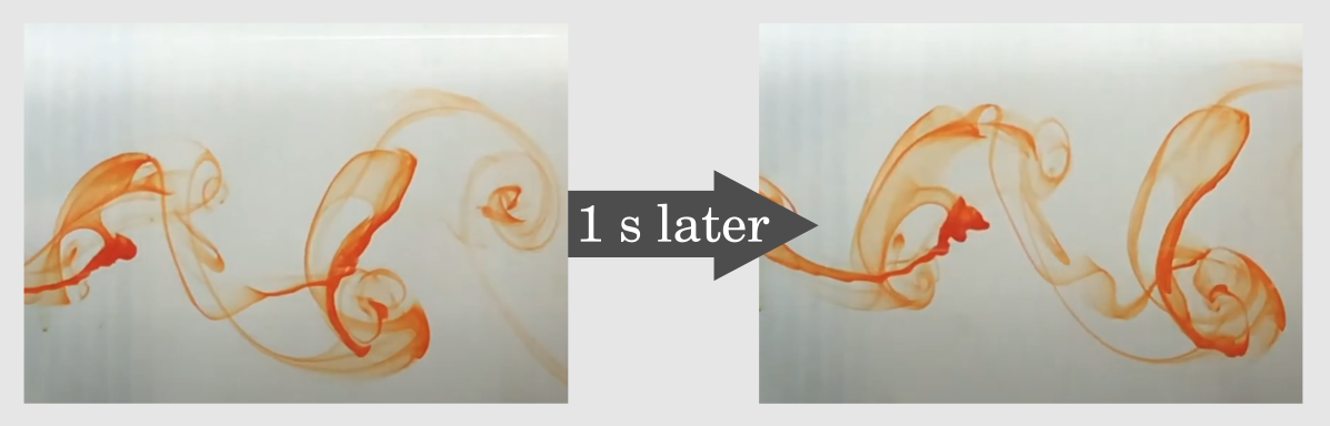
"Beautiful eddies, good-looking flows 👏. And... (Shrug) That's all." --- a guy named Zian Huang

Eddies, and the smaller eddies within them, represent a complex natural phenomenon. It's challenging to describe the intricate motion of a fluid using words alone.

We therefore need a deterministic and systematic way to describe a fluid at a given time ($t$). One powerful method is discretisation, where we approximate our continuous reality. Think of it as applying a mosaic effect to the snapshots above. This approach gives us a way to quantify what we see. For example, we can now say that at the box located at $(10,14)$ on the $x\text{-}y$ plane – 10 boxes to the right and 14 boxes up from the bottom left – the colour intensity fades as time passes. Notice how each mosaic box is represented by a single colour, which is an average of all the colours inside that box. This representation, where each box holds a single value for a fluid attribute, is known as a piece-wise constant configuration.

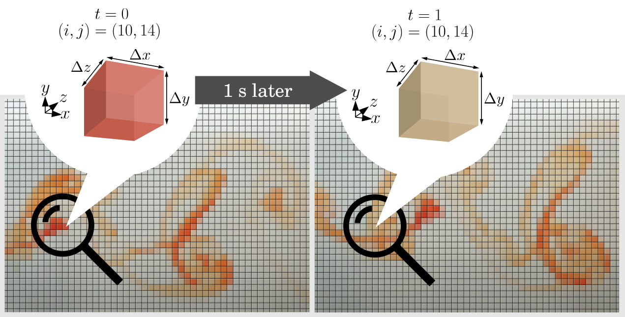
As the size of these boxes shrinks, ($\Delta x \Delta y \Delta z \to 0$), we're moving from a 240p fluid to a 4K fluid and beyond! As the time step drops from $\Delta t = 1$ second towards zero ($\Delta t \rightarrow 0$), it's like we're blinking our eyes faster than a machine gun. As these discrete elements get smaller, our mosaic animation becomes a more realistic representation of the actual flow.

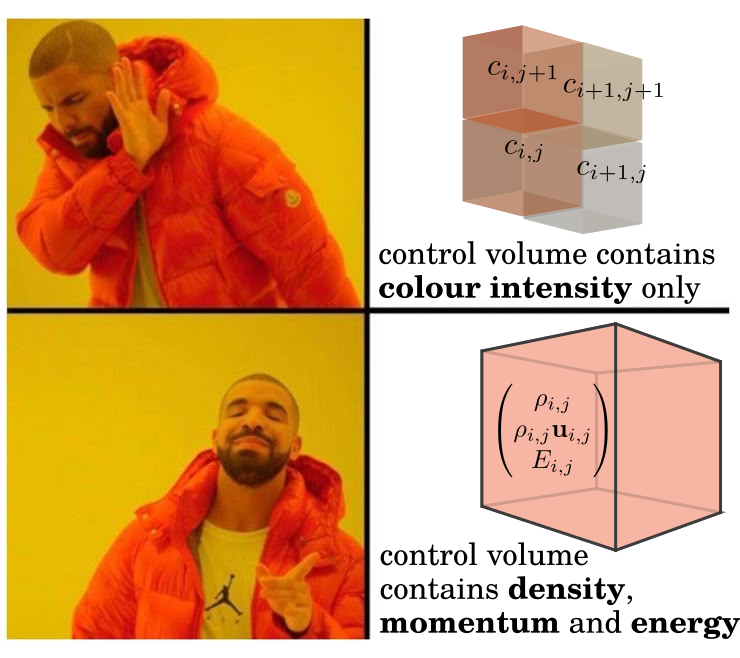
Since we've discretised space and time into boxes and frames, this is the perfect moment to introduce the concept of a control volume. Imagine the fluid we wish to model lives within 3D blocks like those in Minecraft, also known as Cartesian grids. In the example above, these boxes carry information about colour intensity (decreasing from orange to yellow to white). For our purposes, we'll replace colour with the key physical properties of fluid that interest us: density ($\rho$), momentum ($\rho \mathbf{u} = \rho (u, v, w)^T$), and total energy ($E$).

Euler Equations: The Inviscid Holy Grail of Fluid Mechanics

We now have our canvas: a grid of boxes, each filled with fluid properties, waiting to evolve. The next step is to define the mathematical model that governs how these properties change over time.

Our first objective, compressibility, means that density can vary in space. By assuming there are no chemical reactions and that the total mass of the fluid system is conserved, we arrive at the continuity equation:

$$\begin{equation*} \underbrace{\frac{\partial \rho}{\partial t}}_{\text{D1}} + \underbrace{\mathbf{u}\cdot\mathbf{\nabla}\rho}_{\text{D2}} = -\underbrace{\rho \mathbf{\nabla}\cdot\mathbf{u}}_{\text{C1}}, \end{equation*}$$

where the grad operator is defined as $\mathbf{\nabla}=(\frac{\partial}{\partial x},\frac{\partial}{\partial y},\frac{\partial}{\partial z})^T$. The superscript $^T$ indicates the transpose of a matrix.

Term $\textnormal{D1}$ is the local rate of change of density at a fixed point. Term $\textnormal{D2}$ accounts for the change in density due to fluid moving past that point (advection). Finally, term $\textnormal{C1}$ is the essence of compressibility, representing density change due to the divergence of the velocity field. With the help of a negative scaling, intuitively, this expression means that if fluid is gathering (negative $\mathbf{\nabla}\cdot\mathbf{u}$), the density in that region should rise. Conversely, if fluid is spreading out (positive $\mathbf{\nabla}\cdot\mathbf{u}$), the density should fall. This change must be balanced by either a local density variation ($\textnormal{D1}$) or the advection of fluid from neighbouring regions ($\textnormal{D2}$). The presence of $\rho$ to the first power means that as fluid accumulates, density increases linearly.

Using the vector identity $\mathbf{\nabla}\cdot(\rho\mathbf{u}) = \mathbf{u}\cdot\mathbf{\nabla}\rho+\rho\mathbf{\nabla}\cdot\mathbf{u}$, we can rewrite the above to have the conservative continuity equation:

$$\frac{\partial \rho}{\partial t} + \mathbf{\nabla}\cdot(\rho\mathbf{u}) = 0.$$

With density defined, we next consider momentum. This brings us to the holy grail of fluid mechanics: the Navier-Stokes equations. Here, we present the conservative and inviscid form of this equation, known as the Euler equation [3]. The momentum at a point in space changes according to:

$$\begin{equation*} \underbrace{\frac{\partial (\rho u_i)}{\partial t}}_{\text{M1}} + \underbrace{\mathbf{\nabla}\cdot(\rho u_i \mathbf{u}) }_{\text{M2}} = \underbrace{\rho F_i}_{\text{F1}} - \underbrace{\frac{\partial p}{\partial x_i}}_{\text{F2}}, \end{equation*}$$

where: $u_i$ is a velocity component; $p$ is pressure; and $\rho F_{i}$ is a body force (like gravity). The terms are: $\textnormal{M1}$, the local rate of change of momentum; $\textnormal{M2}$, the rate of momentum advection; $\textnormal{F1}$, body forces; and $\textnormal{F2}$, the force due to pressure gradients.

Assuming no body forces, we can rearrange this into the final form of the momentum equation:

$$\begin{equation*} \frac{\partial (\rho \mathbf{u})}{\partial t} + \mathbf{\nabla}\cdot(\rho \mathbf{u} \otimes \mathbf{u}^T + p \mathbf{I}) = 0. \end{equation*}$$

Here, $\mathbf{I}$ is the identity matrix, representing isotropic pressure contribution in all directions, while $\otimes$ is the outer product operator applied on two matrices.

Let's quickly recap. We now have two equations modelling the change in density and momentum:

$$\left\{ \begin{align*} \frac{\partial \rho}{\partial t} + \mathbf{\nabla}\cdot(\rho\mathbf{u}) &= 0\\ \frac{\partial (\rho \mathbf{u})}{\partial t} + \mathbf{\nabla}\cdot(\rho \mathbf{u} \otimes \mathbf{u}^T + p \mathbf{I}) &= 0. \end{align*} \right.$$

A sharp-eyed reader will notice we have a problem: we have three unknown variables $(\rho, \rho\mathbf{u},p)$ but only two equations! To close the system, we need a third equation for energy. We define the total energy per unit volume ($E$) as the sum of kinetic and internal energy:

$$E = \rho\left( \frac{1}{2}\mathbf{u}\cdot\mathbf{u} + e \right),$$

where $e$ is the specific internal energy. To relate this back to our other variables, we assume the fluid is an ideal gas, which follows the ideal gas law:

$$p\frac{1}{\rho}=RT,$$

where $1/\rho$ is the specific volume, $R$ is the ideal gas constant scaled to the number of moles of gas in the specific volume, and $T$ is temperature.

If we further assume the gas is calorically ideal, its internal energy is directly proportional to its temperature. This allows us to establish the relationship:

$$e = c_v T = \frac{R}{\gamma-1}T=\frac{p}{\rho(\gamma-1)},$$

where $\gamma$ is the ratio of specific heats, a constant that depends on the gas. For a diatomic gas like nitrogen, if one dives deep into its molecular structure, one finds $\gamma = 1.4$.

Drawing inspiration from our first two conservation laws, we can write the energy equation as:

$$\begin{align*} &\frac{\partial E}{\partial t} + \mathbf{u}\cdot\mathbf{\nabla}E = -\underbrace{E\mathbf{\nabla}\cdot\mathbf{u}}_{\text{E1}} - \underbrace{\mathbf{\nabla}\cdot(p\mathbf{u})}_{\text{E2}} \\ \implies &\frac{\partial E}{\partial t} +\mathbf{\nabla}\cdot(E\mathbf{u})+\mathbf{\nabla}\cdot(p\mathbf{u})=0 \\ \implies &\frac{\partial E}{\partial t} +\mathbf{\nabla}\cdot((E+p)\mathbf{u})=0 \\ \end{align*}$$

Here, term $\textnormal{E1}$ has the same implication as in the continuity equation: as fluid accumulates, its energy adds up linearly. Term $\textnormal{E2}$ represents the work done by pressure forces.

At this point, we have a complete model governing the dynamics of a compressible, inviscid, and calorically ideal gas:

$$\left\{ \begin{align*} \frac{\partial \rho}{\partial t} + \mathbf{\nabla}\cdot(\rho\mathbf{u}) &= 0\\ \frac{\partial (\rho \mathbf{u})}{\partial t} + \mathbf{\nabla}\cdot(\rho \mathbf{u} \otimes \mathbf{u}^T + p \mathbf{I})) &= 0\\ \frac{\partial E}{\partial t} +\mathbf{\nabla}\cdot((E+p)\mathbf{u})=0, \end{align*} \right.$$

with an equation of state that expresses pressure as a function of our three conserved variables:

$$p(\rho,\rho\mathbf{u},E) = \rho(\gamma - 1)\left( \frac{E}{\rho} - \frac{1}{2}\mathbf{u}\cdot\mathbf{u} \right).$$

"This is indeed quite a journey from that first little whorl 🥵..." --- a guy named Zian Huang

2. How do we solve the model we've just built?

We now have two key pieces: a discretised domain (our 'Minecraft' world) with initial fluid properties contained in each box, and the system of equations that governs them. The goal of this section is to bring them together by discretising the governing equations to fit our gridded space.

A Deeper Dive into Control Volumes and the Finite Volume Method

Conservation is a fundamental principle in physics, and we've already seen its importance in our equations. The central philosophy of the finite volume method, which we'll apply to each box, is based on two key ideas:

(1) Within a control volume, the rate of change of a conserved quantity must equal the net flux of that quantity across the volume's boundaries.

(2) Each control volume is treated as a distinct entity, and the fluid properties within it are represented by a single, volume-averaged value.

From principle (2), we consider the value within each box to be piece-wise constant and uniformly distributed. This is a necessary compromise for modelling the continuous reality of nature on a discrete computer. To implement this, we transform our continuous differential equations into an integral form that applies over a finite volume. Taking the density equation as an example:

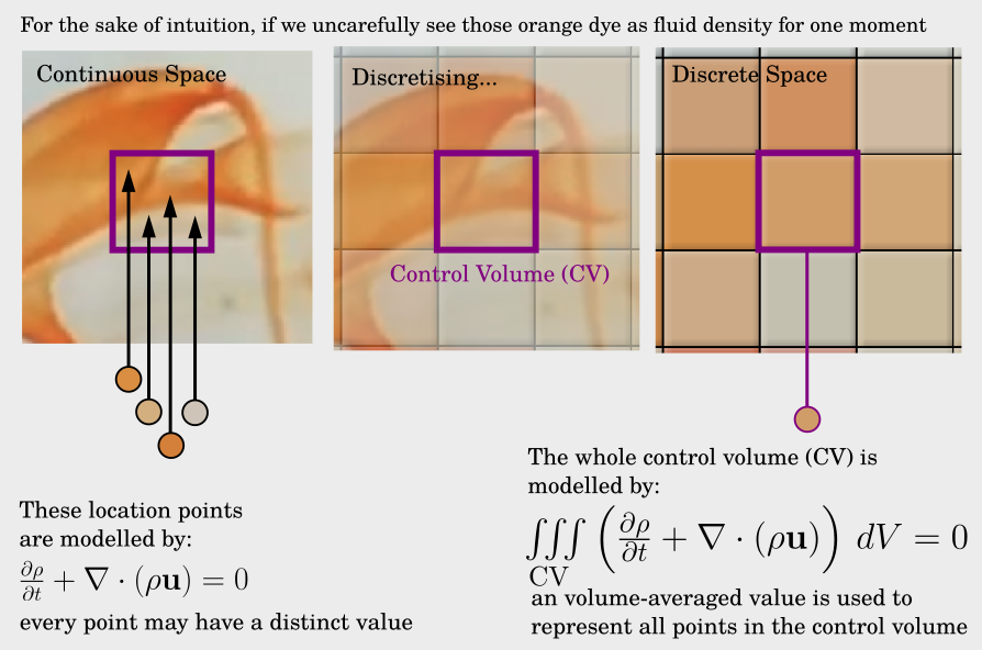
We apply the divergence theorem, $\iiint_{\textnormal{CV}} (\nabla \cdot \mathbf{F}) \, dV = \iint_{\textnormal{S}} \mathbf{F} \cdot d\mathbf{S}$, where $\mathbf{F}$ is a vector field and $\textnormal{S}$ is the surface of the control volume (the 6 faces of the box):

$$\begin{align*} \iiint_{\textnormal{CV}} \left( \frac{\partial \rho}{\partial t} + \mathbf{\nabla}\cdot(\rho\mathbf{u}) \right) \, dV = 0 \\ \iiint_{\textnormal{CV}} \frac{\partial \rho}{\partial t} dV + \iint_{\textnormal{S}} \rho\mathbf{u} \cdot d\mathbf{S} = 0. \end{align*}$$

These two terms perfectly echo principle (1): the first is the rate of change of mass inside the volume, and the second is the net mass flux across its surface.

This process—approximating field values within a volume by a single representative value and enforcing conservation via fluxes at the boundaries—is the essence of the finite volume method.

Since a divergence term appears in all three of our governing equations, we can first rewrite the entire system in a compact vector form [1]:

$$\begin{align*} \mathbf{U}_t + \mathbf{F}(\mathbf{U})_x + \mathbf{G}(\mathbf{U})_y + \mathbf{H}(\mathbf{U})_z &= \mathbf{0}, \end{align*}$$

where $\mathbf{U}$ is the vector of conserved variables, and $\mathbf{F}$, $\mathbf{G}$, and $\mathbf{H}$ are the corresponding flux vectors in the $x$, $y$, and $z$ directions:

$$\mathbf{U} = \begin{pmatrix} \rho \\ \rho u \\ \rho v \\ \rho w \\ E \end{pmatrix}, \mathbf{F} = \begin{pmatrix} \rho u \\ \rho u^2 + p \\ \rho uv \\ \rho uw \\ u(E+p) \end{pmatrix}, \mathbf{G} = \begin{pmatrix} \rho v \\ \rho uv \\ \rho v^2+p \\ \rho vw \\ v(E+p) \end{pmatrix}, \mathbf{H} = \begin{pmatrix} \rho w \\ \rho uw \\ \rho vw \\ \rho w^2+p \\ w(E+p) \end{pmatrix},$$ $$p(\mathbf{U}) = \rho(\gamma - 1)\left( \frac{E}{\rho} - \frac{1}{2}(u^2+v^2+w^2) \right).$$

Let's then consider a single control volume indexed by $(i,j,k)$ at its centre:

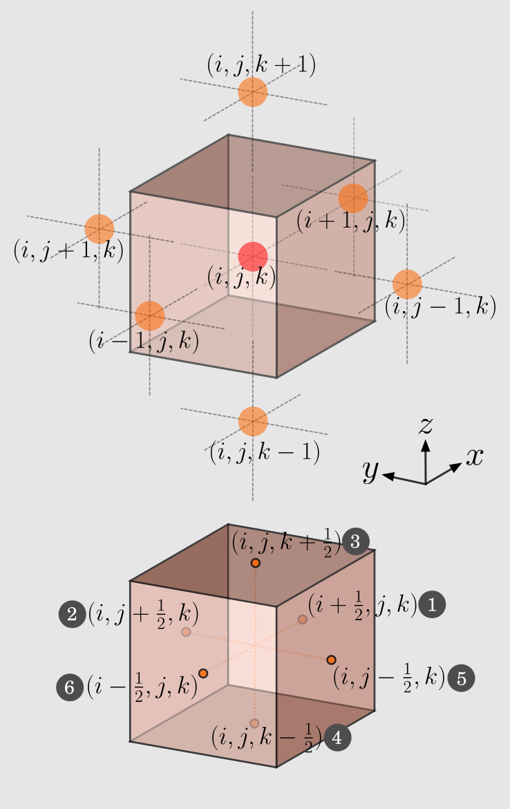
Integrating the vector equation over this control volume and applying the divergence theorem gives:

$$\begin{align*} \iiint_{\textnormal{CV}} \mathbf{U}_t \, dV + \iint_{\textnormal{S}} \Bigl( \mathbf{F}(\mathbf{U}),\ \mathbf{G}(\mathbf{U}),\ \mathbf{H}(\mathbf{U}) \Bigr) \cdot d\mathbf{S} &= \mathbf{0} \\ \\ \iiint_{\textnormal{CV}} \mathbf{U}_t \, dV + \iint_{\textnormal{S}} \mathbf{F}(\mathbf{U}) d{\textnormal{S}_{yz}} + \iint_{\textnormal{S}} \mathbf{G}(\mathbf{U}) d{\textnormal{S}}_{xz} + \iint_{\textnormal{S}} \mathbf{H}(\mathbf{U}) d{\textnormal{S}_{xy}} &= \mathbf{0}\\ \end{align*}$$

Because our values are piece-wise constant, the volume integral becomes the volume-averaged value multiplied by the volume, and the surface integrals become the sum of fluxes over the six faces:

$$\frac{d \mathbf{U}_{i,j,k}}{d t} \, \Delta V + (\mathbf{F}_{i+\frac{1}{2},j,k}-\mathbf{F}_{i-\frac{1}{2},j,k}) \Delta{\textnormal{S}_{yz}} + (\mathbf{G}_{i,j+\frac{1}{2},k}-\mathbf{G}_{i,j-\frac{1}{2},k}) \Delta{\textnormal{S}_{xz}} + (\mathbf{H}_{i,j,k+\frac{1}{2}}-\mathbf{H}_{i,j,k-\frac{1}{2}}) \Delta{\textnormal{S}_{xy}} = \mathbf{0}$$

Here, $\mathbf{F}_{i+\frac{1}{2}}$​​ represents the flux on the face between cell $i$ and cell $i+1$. Now, we approximate the time derivative with a first-order scheme, $\frac{d\mathbf{U}}{dt} \approx \frac{\mathbf{U}^{n+1} - \mathbf{U}^n}{\Delta t}$​, where the superscript $n$ denotes the current time frame. $\mathbf{U}^{n+1}$ indicates the state of fluid attributes at a future time frame $t_{\textnormal{future}} = t_{\textnormal{current}} + \Delta t$. Rearranging to solve for the state at the next time frame, $\mathbf{U}^{n+1}$, gives our final update formula:

$$\begin{align*} \frac{\Delta \mathbf{U}_{i,j,k}}{\Delta t} \Delta x \Delta y \Delta z + (\mathbf{F}_{i+\frac{1}{2},j,k} - \mathbf{F}_{i-\frac{1}{2},j,k}) \Delta y \Delta z \\ + (\mathbf{G}_{i,j+\frac{1}{2},k} - \mathbf{G}_{i,j-\frac{1}{2},k}) \Delta x \Delta z + (\mathbf{H}_{i,j,k+\frac{1}{2}} - \mathbf{H}_{i,j,k-\frac{1}{2}}) \Delta x \Delta y &= \mathbf{0} \end{align*}$$ $$\boxed{ \begin{align*} \mathbf{U}^{n+1}_{i,j,k}=\mathbf{U}^{n}_{i,j,k} &- \frac{\Delta t}{\Delta x}\left(\mathbf{F}_{i+\frac{1}{2},j,k} - \mathbf{F}_{i-\frac{1}{2},j,k}\right) \\&- \frac{\Delta t}{\Delta y}\left(\mathbf{G}_{i,j+\frac{1}{2},k} - \mathbf{G}_{i,j-\frac{1}{2},k}\right)\\ &- \frac{\Delta t}{\Delta z}\left(\mathbf{H}_{i,j,k+\frac{1}{2}} - \mathbf{H}_{i,j,k-\frac{1}{2}}\right). \end{align*}}$$

This approach is known as an explicit time scheme because the future state $\mathbf{U}^{n+1}$ can be calculated directly from the current state $\mathbf{U}^{n}$.

There is one crucial constraint on the size of our time step, $\Delta t$, known as the CFL (Courant-Friedrichs-Lewy) condition:

$$\text{CFL} = \Delta t \left( \frac{|u|}{\Delta x} + \frac{|v|}{\Delta y} + \frac{|w|}{\Delta z} \right) \leq \text{CFL}_{\text{max}},$$

where $\text{CFL}_{\text{max}}$​ depends on the numerical scheme. For the simple scheme we're using, we generally need $\text{CFL} \leq 1$ to ensure the simulation is stable and doesn't 'blow up'. A CFL number close to its maximum stable value helps to minimise numerical diffusion, which keeps sharp features in the flow, like shock waves, from smearing out over time.

Our update equation shows that we can find the state of a cell at the next time frame, $\mathbf{U}^{n+1}$, based on its current state, $\mathbf{U}^{n}$, if and only if we can determine the flux terms ($\mathbf{F}_{i\pm\frac{1}{2},j,k}$​​, etc.) at the cell boundaries.

Gatekeeper: The Riemann Problem

We are just one step away. The final piece of the puzzle is to determine the flux at the boundary between two cells. Let's focus on the boundary between cell $i$ and cell $i+1$ in the x-direction:

Because of our piece-wise constant assumption, there is a sharp discontinuity in the fluid properties at the cell interface! This jump makes it impossible to simply evaluate the flux $\mathbf{F}$ at the boundary, since the properties there, $\mathbf{U}_{i+\frac{1}{2}}$​​, are undefined. Instead, we need a way to calculate the interface flux as a function of the states on the left and right: $\mathbf{F}_{i+\frac{1}{2}}(\mathbf{U}_{L}, \mathbf{U}_{R})$, where $\mathbf{U}_{L}=\mathbf{U}_{i}$​ and $\mathbf{U}_{R}=\mathbf{U}_{i+1}$​. This is known as the Riemann problem.

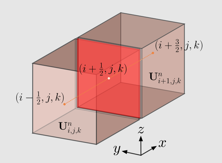
A simple approximate solution is the Lax-Friedrichs flux:

$$\mathbf{F}_{i+\frac{1}{2}}(\mathbf{U}_{L},\mathbf{U}_{R}) = \underbrace{\frac{1}{2} \left( \mathbf{F}(\mathbf{U}_L) + \mathbf{F}(\mathbf{U}_R) \right)}_{\text{F1}} - \underbrace{\frac{1}{2} S_{\text{max}} \left( \mathbf{U}_R - \mathbf{U}_L \right)}_{\text{F2}},$$

with

$$\begin{align*} S_{\text{max}} &= \max(|u_L| + c_L, |u_R| + c_R)\\ c &= \sqrt{\gamma p / \rho} \quad \textnormal{(speed of sound)}. \end{align*}$$

Term $\text{F1}$ is a simple average of the fluxes from the left and right cells. Term $\text{F2}$ is a crucial stabilising term, often called a numerical dissipation or diffusion term. It smooths the sharp jump at the interface by taking an average ($\frac{1}{2}(\mathbf{U}_R - \mathbf{U}_L)$), then scales it by the maximum speed at which information can travel away from the discontinuity ($S_{\text{max}}$​).

One should easily get the remaining $\mathbf{G}_{i,j\pm\frac{1}{2},k}$ and $\mathbf{H}_{i,j,k\pm\frac{1}{2}}$ by considering symmetry, and complete our quest to model the compressible inviscid fluid.

Solving the Riemann problem accurately and efficiently remains an active field of research. For those curious minds wanting more than this simple (but diffusive) approximation, let's look at the structure of the solution to a typical Riemann problem. In practice, it's often more intuitive to think in terms of "primitive" variables: density ($\rho$), velocity ($\mathbf{u}$), and pressure ($p$). The solution evolving from an initial discontinuity develops a distinct wave pattern:

The solution to the Riemann problem typically involves three distinct wave structures moving away from the initial discontinuity:

Understanding the behaviour of these waves is the foundation for developing more sophisticated and accurate Riemann solvers. Prof. Toro's book [1] is an excellent and complete guide to support you on that journey 👍.

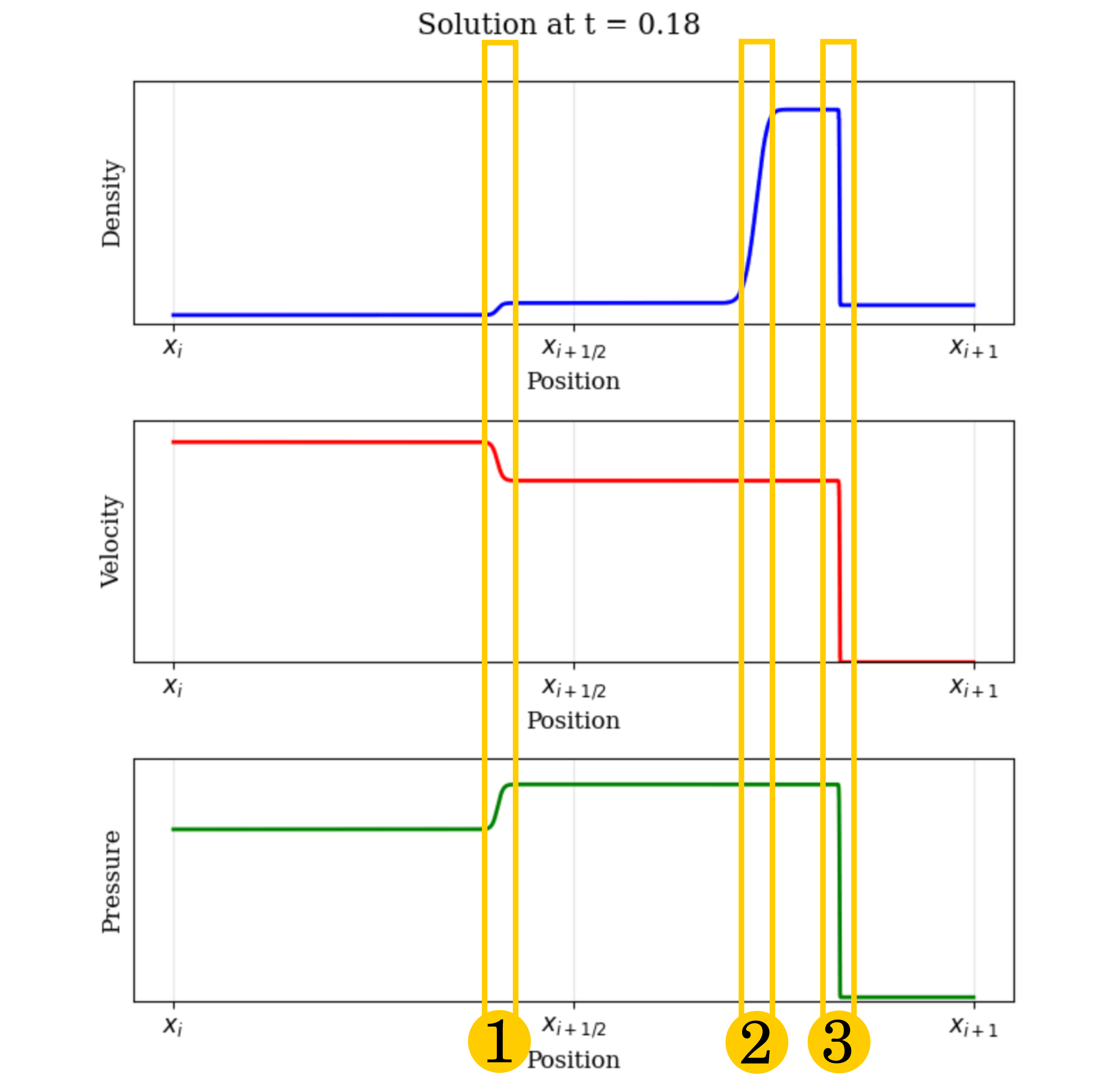
We have come a long way from the first little whorl, even without viscosity

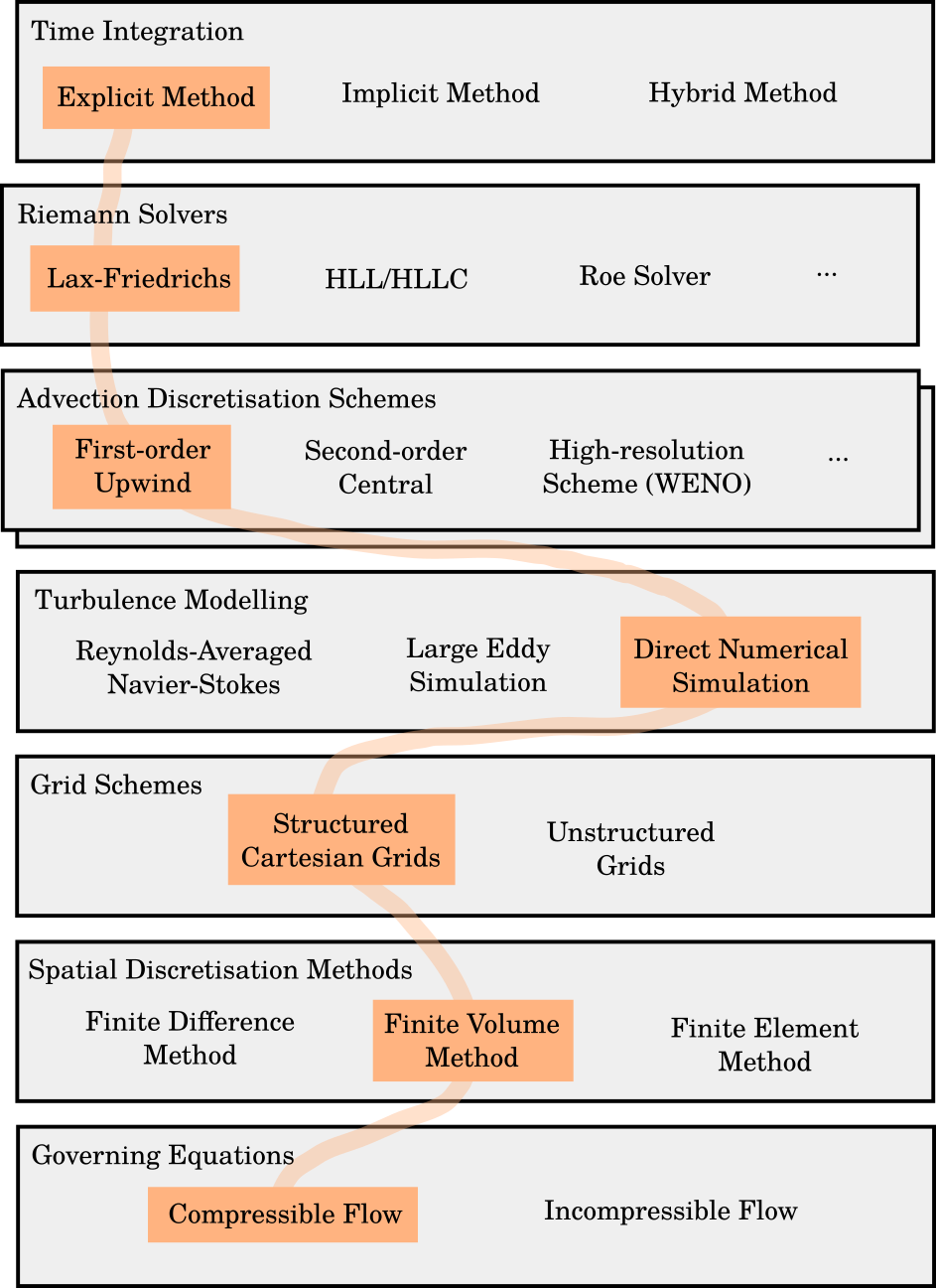
If you've made it this far, thank you for reading! I hope you now feel a bit more knowledgeable about, and interested in, the art of fluid modelling. Lastly, I want to point out the other paths on the broader roadmap of computational fluid dynamics that we didn't take. Some of the choices we made are modular, meaning you can swap in a more sophisticated numerical method for higher accuracy. Others are rabbit holes that lead to entirely new fields of analysis, such as viscous or incompressible flows.

Bon voyage in your fluid modelling quest ⛵.

Reference

[1] E. F. Toro, Riemann Solvers and Numerical Methods for Fluid Dynamics: A Practical Introduction. Berlin, Heidelberg: Springer, 2009. doi: 10.1007/b79761.

[2] Jacob Albright, Flow Visualization in a Water Channel, (Nov. 20, 2017). [Online Video]. Available: https://www.youtube.com/watch?v=30_aADFVL9M

[3] J. H. Ferziger, M. Perić, and R. L. Street, “Basic Concepts of Fluid Flow,” in Computational Methods for Fluid Dynamics, J. H. Ferziger, M. Perić, and R. L. Street, Eds., Cham: Springer International Publishing, 2020, pp. 1–21. doi: 10.1007/978-3-319-99693-6_1.